Here’s an example of how I organize problem sets in a notebook (click to enlarge). I use one notebook for each section and embed them in a OneNote page with the problem descriptions, as well as any illustrations or written work.
Note that each problem occupies one cell—this is to facilitate the next point:
Put this in an initialization cell to scope variables to within one problem:
SetOptions[EvaluationNotebook[], CellContext -> CellGroup]
I usually want any values in the output to have names associated with them to keep everything straight. Put this in an initialization cell:
SetAttributes[saveSet, HoldAll];
saveSet[form : Set[var_, _]] := (lastSet = ToString@Unevaluated@var; form);
saveSet[form : ___] := (lastSet =.; form)

$Pre = saveSet;

$Post = (If[ValueQ@lastSet, Row[{lastSet, " = ", #}], #]) &;
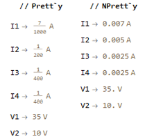
Before
and after:
Solve and NSolve are amazingly useful; they’ll get you through a majority of problems in statics, dynamics, circuits—anything that ends up being a big linear system. We already know we can do algebra; let’s let the CS people flex on us with their work in the crazy-deep world of CASs (Wolfram has a short overview of how they handle algebra and calculus).
Mathematica’s functions (and their error messages) aren’t always the most user friendly, though. If they return anything, they always return a matrix with one solution per row. When I’m doing homework I usually paste a screenshot of the work in MMA into my notes, and a big Mathematica vector kind of ruins whatever kind of readability vibe we’re going for there.

A quick macro helps clean that up a lot. It doesn’t work for Reduce, but if I end up needing something for that I’ll add it here.
Prett`y = (# // Flatten // Column) &;
NPrett`y = (# // N // Prett`y) &;

It took me a long time to realize that the above doesn’t align solutions at the arrows.
Try this instead:
Prett`y[sol_] := Grid[
  (# /. (a_ -> c_) :> {a, "\[Rule]", c} &) /@ Flatten@sol,
  Alignment -> {{Right, Left, Left}}
  ]

Also, my notebook template now includes the helpers ENPrett`y and SPrett`y to convert to engineering and scientific notation.
Why the funny name? I put these in an initialization cell, so they’re defined for the whole notebook; but then I set CellContext→CellGroup, so they aren’t in scope for any of the problems. So we just use fully qualified names to get the y function out of the Prett namespace, mostly because I haven’t found another way to inject globals into each cell context. And Prett`y is easy enough to type.
Solve and Reduce
Ohh boy, this can go on and on. Coming soon
Make a workbook template (or download mine: QuizWorkbookTemplate.nb) and add the following lines to $InstallationDirectory\SystemFiles\FrontEnd\TextResources\Windows\MenuSetup.tr:
Menu["Mathematica",
{
  Menu["&File",
  {
    Menu["&New",
    {
      MenuItem["&Notebook", "New", MenuKey["n", Modifiers->{"Control"}]],
>>    Delimiter,
>>    MenuItem["&Quiz Workbook", KernelExecute[GenerateDocument["path\\to\\template.nb"]], MenuEvaluator -> Automatic, Method -> "Queued", MenuKey["q", Modifiers->{"Control"}]],
>>    Delimiter,
      MenuItem["St&yled Notebook...", FrontEndExecute[{FrontEnd`NotebookOpen[FrontEnd`FindFileOnPath["StylesheetChooser.nb", "PalettePath"]]}]],
(replace "path\\to\\template.nb" in GenerateDocument)
This adds a menu item accessible by alt-f→n→q or ctrl-q; you can change these shortcuts on the MenuItem line.
The default [esc] ... [esc] sequence for Greek letters and special symbols is too far away from the home row. Use this AutoHotkey script to move the esc key under your fourth finger. This is great for Vim too, and probably the only thing my capslock key has ever been used for.
(download script)
SetTitleMatchMode, 2 ; Select any window that partially matches
#IfWinActive, Wolfram Mathematica
Capslock::Esc
After you’ve installed AutoHotkey and saved the script somewhere, place a shortcut to it in one of the startup folders (Windows 10):
C:\Users\<your account>\AppData\Roaming\Microsoft\Windows\Start Menu\Programs\Startup
or
C:\ProgramData\Microsoft\Windows\Start Menu\Programs\StartUp
See Wolfram.com for a complete list of aliases available by default. Many of these are more useful than just naming variables. Some of my favorites are

deg to dimension an angle

ee for Euler's number and p for π

infinity

sums and products
[ctrl-4] and [ctrl-6] to enter the lower and upper limits)

lim (use [ctrl-4] to enter the independent variable)

int and dd for integrals and differentials
[ctrl-5] and [ctrl-6] for lower and upper limits)

transpose

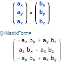
cross product
The apostrophe and backtick characters are reserved in Mathematica, so we can’t directly type a variable name that includes a prime. We can, however, rebind the [esc] ' [esc] (apostrophe) shortcut to enter the unicode character Modifier Letter Apostrophe, which isn’t reserved by the language. Thanks to Jens on StackExchange for this one.
SetOptions[EvaluationNotebook[],
 InputAliases ->
  DeleteDuplicates@
   Join[{"'" -> FromCharacterCode[700]},
    InputAliases /.
      Quiet[Options[EvaluationNotebook[], InputAliases]] /.
     InputAliases -> {}]]
A free bonus for using this character is that it doesn’t look like any reserved character in MMA’s default font, so it won’t hurt readability too much if you know it’s being used.
Solve
Solve and its kin will output SI units by default, even if $UnitSystem is set to Imperial.
There are a couple of workarounds I’ve used for this:
Solve[{
        ...
      }, {...}] /. q_Quantity -> UnitConvert[q, "Imperial"]
The $Post variable is applied to every output expression before it’s displayed.
$Post = # /. q_Quantity -> UnitConvert[q, $UnitSystem] &;
Solve[...]
$UnitSystem is derived from your locale; you can also use "SI", "Metric", or "Imperial".
In the previous section we echoed variable assignments with the name of the variable; here we combine that with automatic unit conversion for the whole notebook.
ShowVariableNames = (If[ValueQ@lastSet, Row[{lastSet, " = ", #}], #]) &;

$Post = (# /. q_Quantity -> UnitConvert[q, "Imperial"] \
      /. Quantity[x_, "BTU"] -> UnitConvert[Quantity[x, "BTU"], "ft*lbf"] &) \
      // ShowVariableNames;
Note that we also convert from BTU to ft·lbf.
If we put the following in an initialization cell then we can set a different automatic conversion for each problem:
Use`SI := $Post = (# /. q_Quantity -> UnitConvert[q, "SI"] &)
        // ShowVariableNames;
Use`FPS := $Post = (# /. q_Quantity -> UnitConvert[q, "Imperial"]
        /. Quantity[x_, "BTU"] -> UnitConvert[Quantity[x, "BTU"], "ft*lbf"] &)
        // ShowVariableNames;

These macros are included in my quiz/homework template.
Hz2 to s-2 in accelerations
Using inverse seconds in equations of acceleration or derivatives can lead to funny output like 10 m Hz^2. When this happens I use
$Post = (# /. Quantity[x_, "Hertz"^(k_: 1)*y_] -> Quantity[x, "Seconds"^-k*y]) &;
Solving big linear systems is one of the more useful things Mathematica can do for engineering homework. I prefer to include units in these systems as a guard against certain easy mistakes. Entering units in MMA is a huge chore, though. The easiest method I’ve found is using [ctrl-=] to use natural language processing through Wolfram Alpha; there’s also the Automatic Units package, but I think it’s still too verbose.
Using the natural language input in MMA is pretty clunky: one keystroke to open the entry, type the value and unit suffix, make sure you enter 12volt because 12V is an airport, press right, wait for the web request to return, press [ctrl-shift-left] to select the block, and finally [ctrl-shift-enter] to evaluate in place. And the box it renders is actually a container, so your arrow keys and text selection don’t work as you expect anymore: the cursor descends into the container instead of stepping over it, and if you click and drag from outside the box, you can’t select any part of the value or unit independently. When we’re doing huge systems for circuit analysis and every constant has a unit, we end up spending most of our time playing with the unit entry box.
The alias below lets you type a unit suffix that’s dissociated from its value, so it behaves like a character and doesn’t interrupt the flow of text navigation. The workflow for giving a value units of Ohms becomes [esc] oh [esc].
{"oh" -> InterpretationBox[
   TemplateBox[{"\[NegativeThinSpace]",
     "\"\[CapitalOmega]\"\[NegativeThinSpace]", "ohms"}, "Quantity"],
   Quantity["Ohms"], Selectable -> False, Editable -> False,
   SyntaxForm -> Mod]},
Let’s break it down:
{"oh" -> ...} creates the rule for oh to be replaced by our box; we’ll include this in our notebook’s InputAliases to get access to the [esc]oh[esc] shortcut.
InterpretationBox defines a 2D renderable element that has one form when displayed and another form when evaluated.
TemplateBox creates a Quantity box with the first list as arguments (these are: value, unit symbol, tooltip string). This lets us use the built-in stylesheet so our box has the same standard form as Quantity. Because it’s wrapped in an InterpretationBox, this TemplateBox will never be evaluated and is just for styling.
The \[NegativeThinSpace] hacks out the margins added by the stylesheet so our box fits more neatly into text.
The second argument to InterpretationBox means that our box will be evaluated as a Quantity with magnitude one.
Setting Selectable and Editable to false cause our box to behave as a single glyph; without these the cursor will descend into the container and the arrow keys won’t behave as you expect.
SyntaxForm gives our box the same evaluation precedence as the actual Quantity box.
We can include this with the alias for primed variables by adding the rules (in curly brackets) as arguments to Join:
SetOptions[EvaluationNotebook[], InputAliases -> DeleteDuplicates@Join[
    {"'" -> FromCharacterCode[700]},
    {"oh" -> InterpretationBox[...]},
    {"V" -> ...}
    ...
Units available in my quiz/homework template: